In this article I will describe a particle simulation that can produce different types of matter based on different input rules. This simulation is based on physical properties and physical rules but the rules were altered in a way that allows for the emergence of intriguing natural-like patterns. The implementation of part 1 and 2 will be done in Processing and the source code will be available at the end. The following illustrations demonstrates a few possible usages for this simulation.
1. Attraction Repulsion between particles
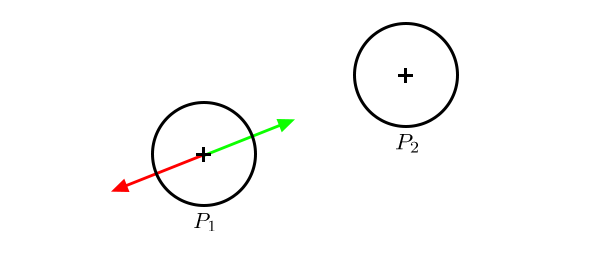
This simulation takes place in a 2d space, although it could also be done in 3D. It is based on attraction / repulsion between a large amount of particles. Each particle of our simulation will be attracted / repelled by the others. We will first cover the mathematics to simulate such phenomena by taking 2 particles  and
and  .
.
Both particles have a position in the 2D space, respectively  and
and  . The following illustration shows the attraction and repulsion forces generated by over .
We will be using Coulomb’s law [1], an experimental law of physics that quantifies the amount of force between two stationary, electrically charged particles of charge  and
and  . The value of and doesn’t really matter in our case, you will see why later. The law of Coulombs states that the force of attraction
  between and is:
![\[F_a = k \cdot \frac{q_1 \cdot q_2}{r^2}\]](https://ciphrd.com/wp-content/ql-cache/quicklatex.com-67c65ec4a9ff6595f5fb4eb4a277e55c_l3.png "Rendered by QuickLaTeX.com")
where
 is the Coulomb’s constant
and
 is the distance between the particles
In our case, we want to control the attraction strength between the particules, and it would be great to do so with a single value. We will consider that all of our particles have the same electric charge  . Thus the formula can be simplified:
![\[F_a = k \cdot \frac{q^2}{r^2}\]](https://ciphrd.com/wp-content/ql-cache/quicklatex.com-d27cb4a1df8b77357032b515fa394c51_l3.png "Rendered by QuickLaTeX.com")
Because and are both constants, we can define them with a single value  , our the strength of the force of attraction between the particles:
![\[S_a = k \cdot q^2\]](https://ciphrd.com/wp-content/ql-cache/quicklatex.com-1b99208cfa21c2f836fa8c0d5a707802_l3.png "Rendered by QuickLaTeX.com")
Therefore our formula can be simplified to the following:
![\[F_a = \frac{S_a}{r^2}\]](https://ciphrd.com/wp-content/ql-cache/quicklatex.com-97c5867e244d8b64294883f3cbcd9545_l3.png "Rendered by QuickLaTeX.com")
The exact same concept can be applied with the force of repulsion, let  be the repulsion strength.
To compute the actual vector of the force of attraction, the operation is simple. We can first compute the direction  between and :
![\[\overrightarrow{D} = \begin{bmatrix}x_{p2} - x_{p1} \\y_{p2} - y_{p1}\end{bmatrix}\]](https://ciphrd.com/wp-content/ql-cache/quicklatex.com-1444f290cf5fe8d547e27e876815d495_l3.png "Rendered by QuickLaTeX.com")
The scalar distance between and will be the magnitude of:
![\[r = ||D||\]](https://ciphrd.com/wp-content/ql-cache/quicklatex.com-30d1528b2b41f1885f1ed1741354f726_l3.png "Rendered by QuickLaTeX.com")
Computing and  is now a trivial task. It can be done by taking the normalized vector of the direction, and multiply it by the scalar value of the force:
![\[\overrightarrow{F_a} = \frac{\overrightarrow{D}}{||D||} \cdot |F_a|\]](https://ciphrd.com/wp-content/ql-cache/quicklatex.com-8a582bcb594ec8dbdcbaf945f8e9c45a_l3.png "Rendered by QuickLaTeX.com")
![\[\overrightarrow{F_r} = - \frac{\overrightarrow{D}}{||D||} \cdot |F_r|\]](https://ciphrd.com/wp-content/ql-cache/quicklatex.com-ef025d44239f822478bcb1a1f2d3cc9b_l3.png "Rendered by QuickLaTeX.com")
Which, in code, translates into:
// compute the force of p2 over p1
PVector D = p2.position.copy().sub(p1.position);
float r = D.mag();
D = D.normalize();
PVector Fa = D.copy().mult(attrStrength).div(r*r);
PVector Fr = D.copy().mult(-repStrength).div(r*r);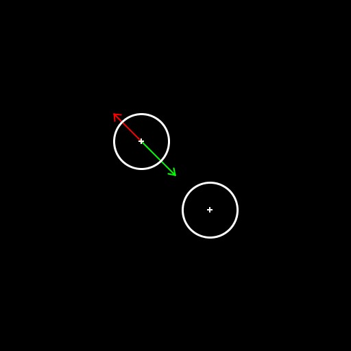
Now that we know how to compute these forces, we can already apply this model to our 2 particles. To update a particle position, we can, on each iteration, compute the sum of the forces applied to it. This sum will be the acceleration. The acceleration can then be added to the velocity, and the velocity to the position. At the end of the iteration, the particle acceleration is set back to 0, and to simulate the friction we multiply the velocity by a scalar factor, the friction decay (0.98 for instance). I already covered this in a previous article, if you are struggling with this step you can check the source code at the end of the article.
For now, we will work in pixel coordinates. Which means that we should take large values for the attraction and repulsion strength for any motion to happen:  and
and  . It is important to note that keeping a repulsion strength higher than the attraction strength will ensure that the particles keep a correct distanciation between them.
Time to throw some more particles in !
We already observe an interesting effect, the particles, over time, tend to get distributed evenly in the space. Before jumping to the next part, let’s introduce a last component to our system. The particles end up being to far away from the center over time. A nice solution is to add some attraction to the center of the world. This is a possible implementation, where the attraction to the center gets higher the further we get from such center:
// we add attraction to the center
p1.acceleration.add(p1.position.copy().sub(center).mult(-0.01));
Let  be the attraction strength towards the center. This is the outcome of this system with the followign values:
| | |
| 110 | 130 | 0.01 |
The particles seems to end up in a sort of vortex over time. This is an interesting behavior, already great ideas could be built from there. This behavior is logical though, think about how gravitation works 🤔
By selecting values carefully for our parameters, we can already get a system that stabilizes himelf:
| | |
| 110 | 130 | 0.001 |
That’s it, these are the very basis for an attraction repulsion system. In the following part, I will propose an idea that allows for more interesting behaviors to emerge.
2. Attraction range and repulsion range
Currently, every particle is affected by every other particle. This is a realistic behavior, however we are not bounded by physics here. We are going to introduce 2 new parameters: the attraction range  and the repulsion range
  . Particles will only be attracted / repelled to each other if the scalar distance between them is under those threshold. Implementation is trivial.
| | | | |
| 110 | 130 | 0.001 | 100 | 90 |
😱 we can already see an interesting behavior with that vortex in the middle only. But let’s explore with some different values…
| | | | |
| 20 | 130 | 0.001 | 150 | 40 |
😱😱 that is even a better vortex than the previous one ! Let’s dig more:
| | | | |
| 20 | 18 | 0.0001 | 40 | 80 |
Hum… there seem to be an issue with those values. Indeed, when particles gets attracted too close, the force generated becomes so high that they end up being sent to the moon. We can fix this issue by adding some collisions to our system.
I will implement a really dumb collision model; it does the job but by no mean is physically correct:
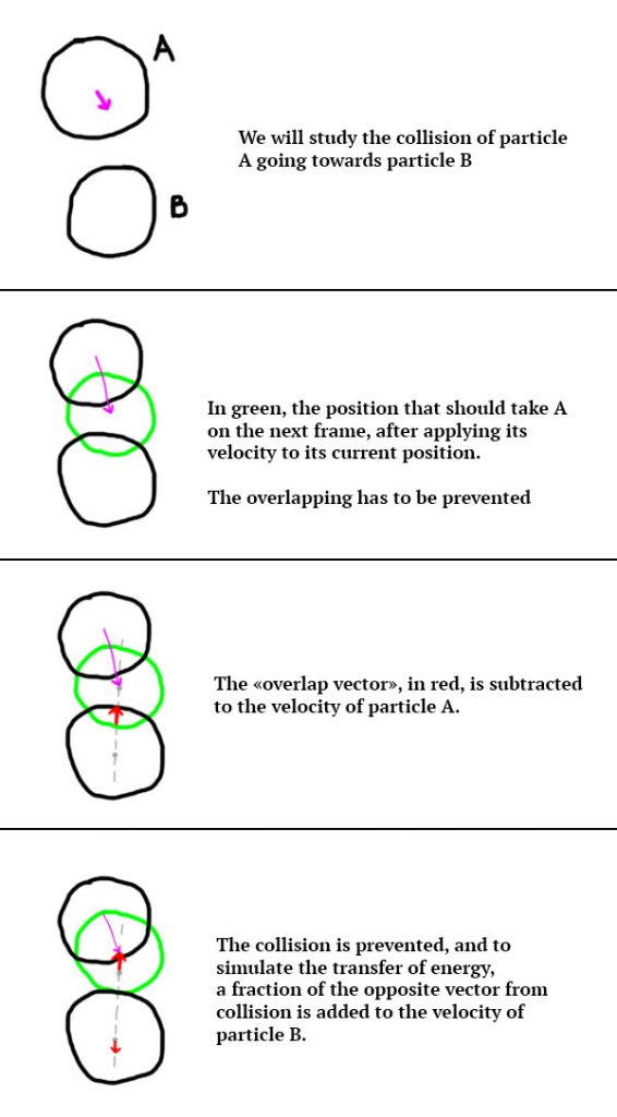
Which translates into the following code:
if (r < p1.radius + p2.radius) {
  PVector mv = D.copy().mult(-((p1.radius + p2.radius) - r));
  p1.velocity.add(mv);
  p2.velocity.add(mv.mult(-0.2));
}
Yeah also I added a radius to the particles that is only used for the collisions and for drawing the particles. It was set to 10 in the following illustration.
😱 BOOM ! Up to our state-of-the-art collision model, the vortex is back !
Please note that 2 more parameters can be added to the list-of-things-we-can-tweak to get funny results: the collision strength  (a factor that indicates by how much a particle should be moved out of another one it overlaps) and the collision response
  (a factor that indicates how much energy is transferred upon collision, it was set to 0.2 in the code above). In the next illustration, I lowered the radius of the particles to 5.
| | | | |  |  |
| 20 | 18 | 0.0001 | 40 | 80 | 0.5 | 0.1 |
Let's try to emphasize this localized behavior. One thing that could be done is to increase the friction. The decay of friction  is currently set to 0.98. By setting it to a smaller value, velocity will decrease faster over time (resulting in increased friction). I will also decrease the maximum velocity
  from 3 to 1.
 |  | | | | | | | |
| 1 | 0.92 | 25 | 18 | 0.0001 | 40 | 80 | 0.5 | 0 |
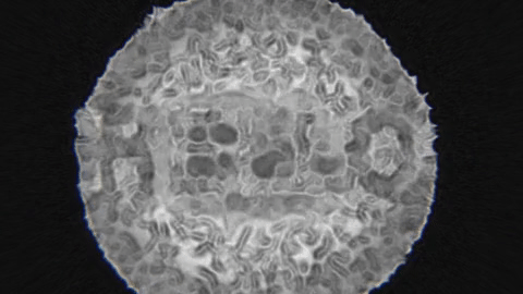
With this particular set of settings, we can observe the emergence of clusters of particles. Beautiful.
| | | | | | | | |
| 1 | 0.92 | 20 | 18 | 0.0001 | 18 | 13 | 0.5 | 0 |
With these settings we get a big cluster of particles. As a quick note, when I work on a new algorithm, this is usually the step where I look back and try to see if pushing it further could be interesting. In that particular case, I think the wide variety of results and the variety of parameters are both indicators that better results could come down the line. So let's dig more.
The next illustration is where this algorithm totally blew my mind. Let's try to find a configuration where particles tend to stick together. For that to happen, I think increasing the friction while keeping a great attraction at a lower than the repulsion could to the trick.
| | | | | | | | |
| 1 | 0.8 | 20 | 30 | 0.0001 | 13 | 20 | 0.5 | 0 |
I was shocked when I saw this. In the middle, some reaction diffusion patterns seem to emerge, however they end up being lost due to the overall repulsion being too high. By increasing the attraction strength just above the repulsion strength, we can ensure that the particles with keep bonding.
| | | | | | | | |
| 1 | 0.8 | 32 | 30 | 0.0001 | 13 | 20 | 0.5 | 0 |
Let's try a slower growth:
| | | | | | | | |
| 1 | 0.2 | 32 | 30 | 0.0001 | 13 | 20 | 0.5 | 0 |
We have some weirdos running around. Honestly I don't know where they come from, I will just ignore them because those patterns are too great. Well as a matter a fact I kinda know where they come from: particules which were randomly placed on top of each other at initialization. One solution could be to only compute the forces between 2 particles if their distance is higher than 0.5.
And let's throw some more particles in, 800. I also increased to friction decay to 0.95 to get some motion back.
At this point, the next step on the line is to scale this system up. 800 particles is fun, but going to higher scales would destroy the CPU. There are optimizations that could be made, such as storing the particles in a grid and only compare particles from adjacent cells. And other less naive approaches. OR the computations could be moved to the GPU, by using compute shaders.
The source code of the implementation on Processing, up to this point, is available on Github:
https://github.com/bcrespy/LocalizedAttractionRepulsion
3. Scaling this system up
Compute Shaders [2] have the ability to store small chunks of data into the GPU memory, that can be shared across the different cores of the Graphics Card. I won't go into details in this article because it is out of the scope, you should know that usually, when it comes to particles interacting with each other, Compute Shader can increase performances by a lot.
The following illustrations were generated using the same algorithm presented above. The only difference is the scale of the space in which the particles evolve, it is not in pixel coordinates but is within [-2; 2]. This is why the overlay values are much smaller than the ones presented before.
The particles are colored based on the magnitude of their velocity from white (no velocity) to red (high velocity). The number of particles is 12 544, and each particle interacts with each other particle.
Because this simulation relies on particles, we can interact with the particles easily. In the following illustrations, a vector field is generated from a point that moves in the space. Basically, particles are repelled by this point. I used it to show you that this simulation mimics the behavior of liquids, which is pretty neat.
I used this technique when I did some visuals for Inkie. I layered many other techniques to get this particular look / interactions with the lasers, but the idea remains the same:
I have also explored this system furthermore on my instagram:
Follow me on instagram for more contentThat will be it for this article. Thanks for reading through, I hope you will find some inspiration in that technique and build your own stuff with it 👽
Link to the repo of the Processing project:
References
- Coulomb's law, Wikipédia
- Compute Shaders, Khronos